Output filter
Output filter
The created signal can be output after applying a filter (FIR filter) with arbitrary frequency characteristics.
You can also create a signal with an integral multiple of the specified format and then filter it. (Oversampling)
* You can also change the characteristics of the filter during signal generation.
Check the Filter check box ![]() to activate the filter.
to activate the filter.
When checked, it changes to ![]() and the filter setting window is displayed.
and the filter setting window is displayed.
The filter is enabled only when the filter setting window is displayed.
Filter Settings window
The frequency characteristics of the filter can be set / changed.
(The size of the window can be changed freely.)
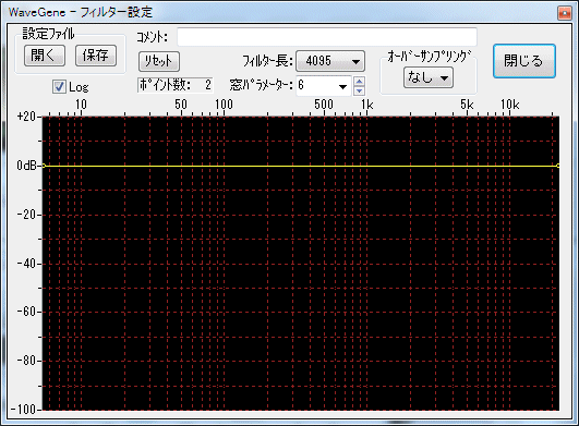
- Edit control point (points)
It is a bending point that determines the curve of the frequency characteristic of the filter, and it has a frequency and the amplitude (gain) there.
(Hereafter abbreviated as Point)
In the state in which the initial state filter is not applied, the gain is both 0 dB at the left end (0 Hz) and the right end (sample frequency / 2) as shown above. (Flat in all bands)
By editing the number of points and the frequency / gain, set a curve of arbitrary frequency characteristics.
- Import and save configuration file (filter parameter file)
The current filter setting is saved in the WG.INI file at the end of WG.EXE together with the waveform parameters etc. without doing anything, and it is reproduced on the next start.
When you want to save it separately, you can reproduce it at any time by saving it as a filter parameter file (*. WGF) with a name given to the current setting.
With the Open , Save button in the configuration file group box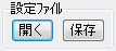 , You can read and save the filter parameter file.
When saving, it is convenient to write a comment for explanation in the comment edit box.
(Comments and parameters are saved in the file)
* You can also load filter parameter file (*. WGF) by dropping it on this window. - Toggle vertical axis (amplitude / gain) display
Change the setting of the scale dB max (+ 40 to 0 dB) of 0 dB or more and the scale dB min (-20 to -160 dB) of 0 dB or less in the pop-up menu displayed by right-clicking the mouse in the scale display area on the vertical axis can.
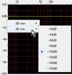
Point setting / movement by dragging the mouse is limited to the upper and lower limits of the display area.
Therefore, if you use only 0 dB or less, setting dB max to 0 dB always fixes the upper limit to 0 dB, making it easier to set up and convenient.
- Toggle horizontal axis (frequency) display
![]() If the check box is checked, logarithmic display will be displayed, if not checked linearly.
If the check box is checked, logarithmic display will be displayed, if not checked linearly.
- Reset properties and check the total number of points
Reset button you can reset the filter settings.
The total number of current points is displayed below the reset button.
When reset, the point for determining the characteristic (curve) of the filter is initialized to two ends of the band (0 Hz and sampling frequency / 2), and the flat (gain 0 dB) characteristic. - Filter Length
In the Filter Length combo box, you can change the length (order) of the coefficients of the filter.
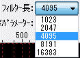
A larger sharper blocking becomes possible, but as a matter of course the load on the CPU becomes larger, it is better to reduce it when there is no need for a sharp change.
The length of the internal calculation buffer will be the length of this setting + 1, and the calculation of the filter will also be calculated in this length unit.
Actually, filter calculation (convolution) is done with FFT twice the length.
(This FFT is required twice for each channel)
The resolution of the filter's frequency axis is the sampling frequency / (filter length + 1).
For example, at 48000 Hz sampling with filter length 4095, it becomes 48000/4096 = 11.72 Hz, and point setting / movement is possible only at this multiple frequency position.
If the frequency axis display is logarithmic display (Log), changing the filter length will change the minimum frequency of display accordingly.
Note :
In the case of logarithmic display, in principle 0 Hz can not be displayed, but for the sake of convenience, the position which is half of the frequency of the resolution of the filter, which is the lowest frequency that can be set, is 0 Hz (Left end) is displayed.
- Window parameters
Window Parameters Combo box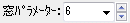 to determine the shape of the Kaiser window used for filter design You can change the value of the variable.
Values range from 0 to 10, you can directly set any value other than the preset value.
(You can also change it with 0.1 steps with the right up / down control.)
The larger the value, the sharper the cutoff becomes possible, but the spread from the point becomes large, so it is good to set it while checking the actual frequency characteristics (see below).
* _char_ may be expressed as _char_.
In that case, _char_ = _char_ * _char_ 'and ' _char_ is the value before multiplication by _char_.
The Kaiser window has a shape resembling the existing window depending on the value of _char_.
_char_ = 0: rectangular window (no window) _char_ _char_ 5: Hamming window _char_ _char_ 6: Hanning window
_char_ ? 9: Blackman window - Oversampling
If the oversampling combo box is set to none it is only filtered, but here none ( x 2 < If you set it to, x4 , x8 , x16 ), you can create a signal with that multiple sampling frequency and then filter I can do it.
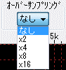
For example, if you specify x16 when formatting with a sampling frequency of 48 kHz, create a signal with a sampling frequency of 48 x 16 = 768 kHz and set it here A band-limiting filter (decimation filter) of a frequency characteristic that passes only up to 48/2 = 24 kHz is thinned out, and sampling frequency It is returned to the 48 kHz signal.
It is possible to suppress out-of-band components of unrestricted waveforms other than sine waves, and to create high-quality noise.
(If you generate M series noise at about x 8 and apply decimation filter, you can create high quality white noise
Also, at that time, filtering with a frequency characteristic of -3 dB / oct (-10 dB / dec) in the whole band results in pink noise.
Noise of any other characteristic can be created in the same way)
* As the multiplier is increased, the computation time increases, so if you try to play it in real time on a non-powerful CPU, you may skip the sound.
In that case please write it to the wave file once and use it.
(Currently the program is not particularly speeded up, but it may be faster in the future)
note:
Even if it is set to something other than none (x2, x4, x8, x16), the signal is re-created at that multiple sampling frequency and then filtered, so the frequency of the created signal is the same as when the filter is not applied Hmm. (It is only bandwidth limited)
Also, it does not mean that the sampling frequency is raised by inserting data of zero as much as the original data.
For example, if you create a 1 kHz sine wave with none at a sampling frequency of 48 kHz, x 2 will create again at twice the sampling frequency 96 kHz and decimate it, It returns to 1 kHz of the same 48 kHz sampling as the original.
However, only the user waveform is handled specially.
As it is not possible to re-create the data with the user waveform newly, if you set the sampling frequency of x 2 , the frequency will be doubled, the playback time will be halved fast? It will become.
In this case, it lacks consistency with other signals, so only overwhelming user waveforms are inserted at the oversampling by zero, so that the playback frequency is not changed.
That is, it acts as an interpolation filter.
* oversampling tricks (file creation)
(It's not even a thing like that ...)
Normally, even if you create a wave file with x2, x4 ... as above, the format of the completed file will be restored and the sampling frequency will be It will not be x2, x4 ..., but if you do the following, the file with the sampling frequency in the state of x2, x4 ... (before decimation of data by multiplying only the decimation filter) You can create.
* ![]() Press the output button to Wave file , and output to " Wave file " Hold down Ctrl key and press the " Save " button when you press the " Save & , You can create a wave file in the format of x2, x4 ....
Press the output button to Wave file , and output to " Wave file " Hold down Ctrl key and press the " Save " button when you press the " Save & , You can create a wave file in the format of x2, x4 ....
Note: Pressing the Ctrl key is not the time to press the Output to Wave File button.
This is when you press the " Save " button in the subsequent dialog box for specifying the file name.
(You can release Ctrl key when file creation starts)
Also, only Wave files can be created.
You can not create a text file (*. WGT) in the x2, x4 ... format by pressing the Output to Wave File key while holding down the Shift key.
* Sampling frequency conversion (interpolation) of Wave file
Using this trick, it is possible to convert the sampling frequency of the wave file, although it is only x2, x4, x8, x16.
* After loading the wave file you want to convert to the user waveform, set the oversampling setting to x2, x4, etc. Wave file length / sweep length combo box by setting the length (sec) of the read file with ![]()
![]() Output to Wave file By clicking the button , you can create a Wave file whose sampling frequency has been converted.
Output to Wave file By clicking the button , you can create a Wave file whose sampling frequency has been converted.
Always Ctrl key while pressing the " Save " button in the file name designation dialog.
Also, do not forget to set the sampling frequency of the WG creation format to be the same as the value of the loaded file, and reset the filter characteristics to flat.
- Close button

Close the filter setting window.
It is also possible to close the setting window by unchecking the filter check box in the main window I can do it.
Editing filter frequency characteristics
- Set curves of arbitrary frequency characteristics by editing the number and frequency / gain of edit control points (points).
* The point editing method is almost the same as other waveform editing software. - Review and move points
When placing the mouse cursor over a small ○ indicating a point, the cursor changes to a crosshair cursor, and the frequency and gain of that point are displayed in a small floating window. (The color of the floating window also turns yellow.)
You can move the point by dragging the mouse as it is, and follow the display of frequency and gain.
In the above example, since it is in the initial state immediately after resetting, neither point can change the frequency only by the gain, the frequency can not be changed.
- Create point
You can create a new point there by clicking the left mouse button in a place without a point.
It is possible to move by dragging as it is, and the point of the newly created point can change the position of the frequency unlike points at both ends.
However, it is not possible to move to the position of the frequency exceeding the point of both neighbors only by the allowable range.
* The minimum spacing of points is the resolution of the filter, ie sampling frequency / (filter length + 1).
Up to 100 points can be created for points.
- Edit point
Right-clicking the mouse on the point will display a pop-up menu like the one below.

When you select [1] edit , the point editing window opens and you can enter the frequency and gain of the point numerically.
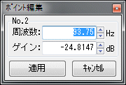
For convenience, the left end (0 Hz) is numbered as No.1, and the frequency increases to No.2, No.3 ... in the right direction.
* Frequencies can only be set in multiples of the resolution of the filter.
Even if you say it is difficult to calculate yourself, you can enter the frequency you want to set in the edit box appropriately.
It is automatically changed to a multiple of the resolution about 1 second after the key input end.
Moreover, it can not set to a value exceeding the frequencies of both neighboring points.
You can change it even with the up / down control ![]() but in this case it is always a valid numeric value that is an integer multiple of the resolution.
but in this case it is always a valid numeric value that is an integer multiple of the resolution.
* Regarding the gain, it is only from dB max to dB min set on the scale on the vertical axis of the graph, but if necessary it is possible to enter a wider range of values.
So, for example, although it is virtually meaningless in practice, if you want to set the gain to infinity - zero (zero signal) - you can set it to -200 dB or -300 dB.
However, on the graph display, ○ is displayed at the upper limit dB max or lower limit dB min of the range of the current display area.
Therefore, although it may be displayed quite differently from the actual inclination, the curve of the internal filter is accurately calculated.
Furthermore, it is certain to check actual frequency characteristics (described later).
[2] Delete , the point will be deleted.
* Of course you can not delete points at both ends.
[3] Choosing to the next point will bring up a further pop-up menu.
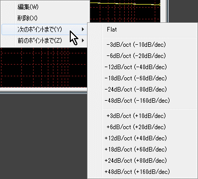
By selecting these menus, you can connect up to the point on the right of the current point (the one with the higher frequency) with the line of the specified slope [flat, attenuation, increase] The gain of the point is changed.
For example, as in the example below, when the left point is 105.5 Hz - 20 dB, and the right point is at the frequency 10 times that frequency
 The left point is 105.5 Hz - 20 dB
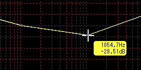 The right point is 1054.7 Hz -28.51 dB
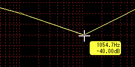
If you select -6 dB / oct (-20 dB / dec) to the next point at the left point, the gain of the right point will be changed to -40 dB.
The same is true when you want to make other slopes, and if you want to make both gains the same, you can choose Flat.
* For example, if you want to set the slope to -3 dB in all bands, it is possible to select -3 dB / oct (-10 dB / dec) to the next point at the 0 Hz point at the left end immediately after resetting.
If you filter the white noise with this filter, it will become pink noise.
If you apply a filter of -6 dB / oct (-20 dB / dec), it will become Brown noise.
(Since the overall gain goes down, it is a good idea to raise the gain of 0 Hz to the extent that the peak of the output signal does not exceed 0 dB beforehand)
Note: When calculating the gain slope as in this case the point of 0 Hz is actually the lowest frequency (the frequency of the resolution) Half of the frequency point It will be treated as special. (Correction for Log scale)
[4] To the previous point changes to specifying the inclination to the point next to the left with the point on the right as the base point, otherwise it is exactly the same as above [3] is.
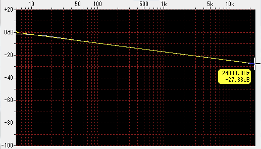
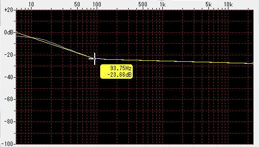
Actual frequency characteristics of the filter
Even if you set a point and set the curve of the desired frequency characteristic, the frequency characteristics when actually operating as a filter will not be as per the curve.
For that purpose, the filter coefficients (impulse response) require infinite length, but in reality naturally it is limited.
Especially if you give sharp changes to the setting curve, the actual characteristics deviate greatly from the set curve.
Actual frequency characteristics vary depending on the setting of filter length and window parameters, but it is convenient as it is designed to display in real time the frequency characteristics actually obtained to make it easier to design the desired characteristics.
Even if the position of the point is moved, the actual frequency characteristics will be displayed following the change in real time.
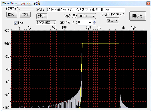
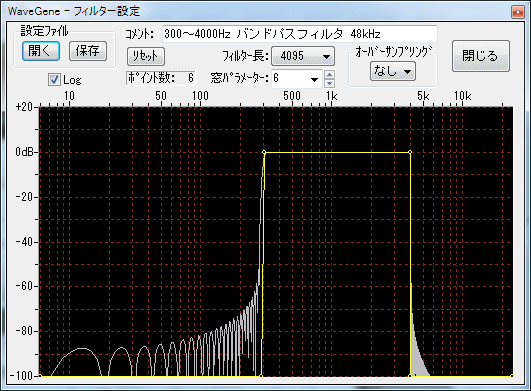
- It is an example of a band pass filter of 300 to 4000 Hz.
It is the curve set to be displayed in yellow, and the actual frequency characteristic is displayed in gray.
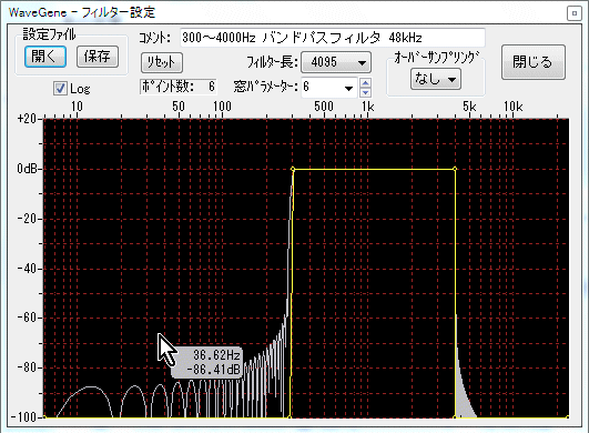
When you move the mouse cursor on the graph, the gain of the actual characteristic at that frequency position is displayed as a floating window (gray).
If you move the mouse cursor to a point, the cursor will change to a cross (the color of the floating window also turns yellow), and the point setting value will be displayed.
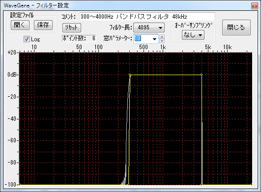
- It is when the window parameter is changed.
When the window parameter is 0. (It is the same as not hanging the window)
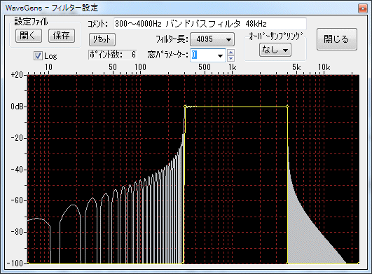
When the window parameter is 10.
- This is when you change the filter length.
For filter length 2047.
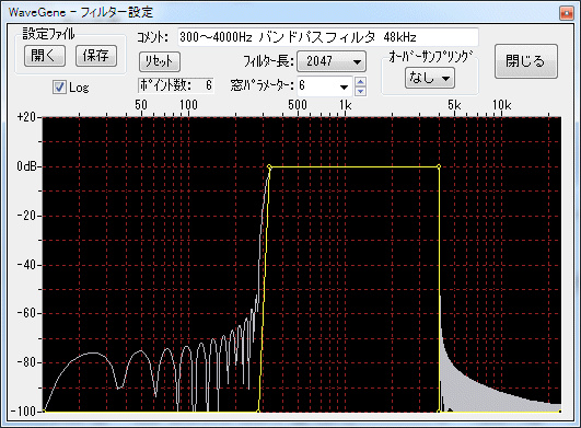
In case of filter length 8191.
Changing filter characteristics during signaling
- You can change the filter characteristics when
button is pressed to generate a signal, that is, even during operation ![]() I will.
I will.
You can try filtering it while sounding such as white noise and move the peak of its frequency characteristics.
However, please be aware that the load on the CPU increases by that much, so skipping may occur depending on the environment.
In addition, since it changes only in units of length of filter length + 1 (corresponding time), if the filter length is increased to cause a very sharp temporal change, the amplitude becomes discontinuous depending on the change of the frequency characteristic In that case, please be aware that you will naturally hear it as a petit noise at that position.
Other
- When editing a point, when the frequency axis is Log display, the point interval becomes narrower in the high frequency part, so it is better to remove the Log check and make a linear display It becomes easy to do.
- When switching the frequency axis to linear display, the curve connecting each point is displayed as a straight line for convenience, but note that the gradient in the linear scale is not the slope of the actual filter characteristic stay here.
The change in the actual frequency characteristic of the filter is calculated so as to be the slope of the line displayed at the Log scale only, so it will not be a straight line at the linear scale. (Exponential curve)
Please confirm with the actual frequency characteristic to be displayed.
* It is not possible to make such a filter characteristic that it becomes the inclination of a straight line as a linear scale. - Filter frequency resolution is sampling frequency / (filter length + 1).
However, the characteristics of the window function are added, and the actual resolution slightly expands on both sides of the center frequency.
For example, if you only want to cut out components of a certain frequency, you should set not to cut only the point of that frequency but to cut it by slightly expanding both sides.
Adjust while confirming actual frequency characteristics with filter length and window parameter value. - Characteristic setting of the filter, that is, the setting of the frequency position of each point, depends on the sampling frequency as described above.
Therefore, when setting a filter (for example, 10 kHz low pass filter) with an absolute fixed frequency, it is necessary to set the point of the filter for each sampling frequency.
When the sampling frequency is changed from the design time, a confirmation message is displayed as to how to convert the frequency position of each point.
When changing the filter designed at sampling frequency 48 kHz to 96 kHz and trying to use it, a message box like the one shown below will be displayed.
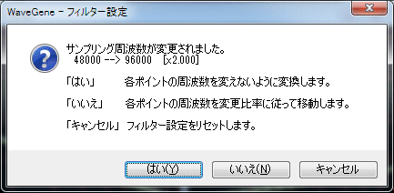
If you press Yes , only the internal parameters are converted so that the set frequency of each point does not change the original frequency value. (Gain does not change)
When you press No , the setting frequency of each point is moved relative, and in this case, everything is doubled. (Gain does not change)
Press Cancel to change to the reset state (flat) at 96 kHz.
Please be aware that the cancellation is a reset.
Even when * yes , since the resolution of the filter changes, the frequency may change slightly due to that limitation.
If you want to set it strictly, please confirm after conversion and reedit if necessary.
- Format of filter parameter file (*. WGF)
The filter parameter file has the following text format.
Example: 300 to 4000 Hz band pass filter (in the setting example below)
"WaveGene Filter Parameter", 1.00 ← 1st line title and version
"Comment", "300 to 4000 Hz band pass filter 48 kHz" ← Comment
"OverSampleRate", 1 ← oversampling rate
"Size 1", 4096 ← filter length + 1
"AmpScale_dB_Max", 20 ← Value of amplitude scale dB max
"AmpScale_dB_Min", - 100 ← Value of amplitude scale dB min
"KaiserAlpha", 6 ← value of window parameter
"Sampling Frequency", 48000 ← Sampling frequency
"Points", 6 ← number of points
; No. | Indx | Frequency | Amp.dB ← Description Comment line
1, 0, 0, -300 ← or less, No, frequency index, frequency and gain dB value of each point are repeated.
2, 25, 292.96875, -300
3, 26, 304.6875, 0
4, 341, 3996.09375, 0
5, 342, 4007.8125, -300
6, 2048, 24000, -300
Since it is a text file, it can be edited with a text editor.
The frequency index indicates the position of each point at the sampling frequency / Size 1, which is 0 to Size 1/2. - Drawing of the actual frequency characteristic is usually calculated at the frequency position of the fineness of 8 times the frequency resolution by the filter length.
If you have enough CPU processing speed and want to display it in more detail, after terminating temporarily, add the following description to any position in the Filter section of WG.INI and reexecute it.
[Filter]
ResponseRate = 16
4, 8, 16 can be specified.
If it is set to 4, the display becomes rough but the CPU load decreases.
Even if it is 4, the intermediate peak and dip positions are displayed properly, so there is no problem in practical use.
Configuration example
- [Example 1] 300 to 4 kHz bandpass filter
It is just a band pass filter.
48 kHz 6 points
|
No. |
Frequency |
Amp.dB |
|
1 |
0 |
-300 |
|
2 |
292.96875 |
-300 |
|
3 |
304.6875 |
0 |
|
4 |
3996.09375 |
0 |
|
5 |
4007.8125 |
-300 |
|
6 |
24000 |
-300 |
Changing the filter length and window parameters will change the actual characteristics.
If you want to use a filter that is not steep like this, add more points and make it gentle.
- [Example 2] 15 kHz low pass + 50 u s emphasis
FM broadcast This is a filter applied to a wave file for compositing signal.
50uS emphasis is a rough approximation. For the emphasis, the overall level has been lowered by 1 dB.
44.1 kHz 8 points
|
No. |
Frequency |
Amp.dB |
|
1 |
0 |
-1 |
|
2 |
495.2636719 |
-1 |
|
3 |
1001.293945 |
-0.5 |
|
4 |
2002.587891 |
1 |
|
5 |
3176.147461 |
2 |
|
6 |
14997.87598 |
12.5 |
|
7 |
15008.64258 |
-300 |
|
8 |
22050 |
-300 |

Created with the Personal Edition of HelpNDoc: Create iPhone web-based documentation